Wordle Words and Expected Value

Like many people, I’ve gotten sucked into wordle. For those unfamiliar with the game, you are tasked with identifying a five-letter word. You input a guess (which must be a five-letter word) and are told whether each letter in your guess is:

1. not in the word (black square)
2. in the word but in a different position (yellow square)
3. in the word and in the correct position (green square)

You have six guesses to figure out the correct word.

Think Wheel of Fortune but with the requirement you buy bundles (words) of letters.

Unlike most people who can just enjoy a word puzzle, it immediately made me start to wonder “what is the best first word you can play?”

So I went and acquired a helpful list of ~479,000 words in the English language intended for spell-checking, posted on GitHub. We can discard any words with digits or other symbols in them as well as any words that are not exactly five characters long. This leaves us 15,918 possible words that are five characters long and in the English language.

I decided to compute a word’s value using three measures

1. What is the expected number of green squares
2. What is the expected number of yellow squares
3. What is the expected number of yellow or green squares

when guessing that word.

I got started by pulling the word list from GitHub:

words <- read_lines("https://raw.githubusercontent.com/dwyl/english-words/master/words_alpha.txt")

And reducing to only those with exactly five characters:

five_letter_words <- words[stringr::str_length(words) == 5]

Next, for each letter a to z, I found the frequency with which it was yellow or green for each character position 1 to 5. Forgive the loop - it’s the weekend:

letter_matches <- vector("list", 26)
for (letter_index in 1:26) {
  letter <- letters[letter_index]
  matches <- vector("list", 5)
  for (character_index in 1:5) {
    matches[[character_index]] <- tibble(
      letter = letter,
      yellow_or_green = stringr::str_detect(five_letter_words, letter),
      green = stringr::str_sub(five_letter_words, 
                               character_index, 
                               character_index) == letter
    ) %>%
      mutate(
        yellow = yellow_or_green & !green
      ) %>%
      select(letter, yellow, green) %>%
      mutate(
        character_index = character_index
      )
  }
  letter_matches[[letter_index]] <- matches %>%
    bind_rows()
}

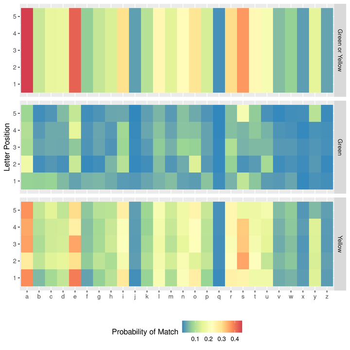
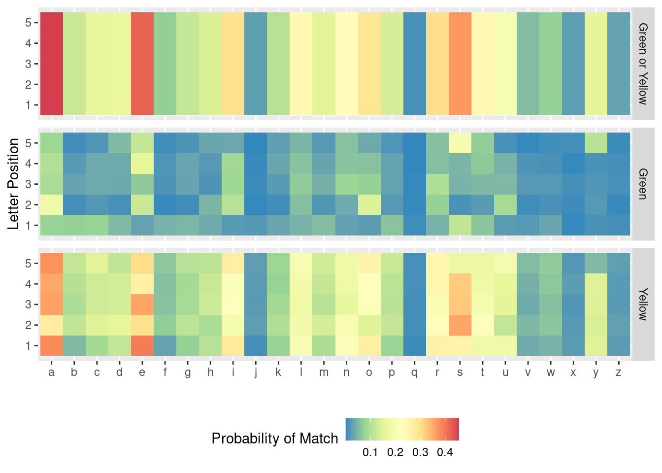
We can then see the estimated probability that a given position is a particular letter (green) or that the word features the letter in another position (yellow):

letter_matches %>%
  bind_rows() %>%
  group_by(
    letter, character_index
  ) %>%
  summarize(
    `Yellow` = mean(yellow),
    `Green` = mean(green),
    `Green or Yellow` = mean(green | yellow),
    .groups = "drop"
  ) %>%
  gather(color, prob, -letter, -character_index) %>%
  mutate(color = forcats::fct_relevel(color, "Green or Yellow")) %>%
  ggplot(aes(x = letter, 
             y = character_index,
             fill = prob)) + 
  geom_tile() + 
  facet_grid(rows = vars(color)) + 
  labs(x = "", 
       y = "Letter Position", 
       fill = "Probability of Match") + 
  scale_fill_distiller(palette = "Spectral") + 
  theme(legend.position = "bottom")

Largely, this is not surprising. Vowels are more likely to occur than other letters. Some things stand out, such as “s” or “y” being likely to be the final letter in the word. The letters “a”, “e”, and “s” seem like good letters to include in the guess.

Next, I used these probabilities to compute the expected number of green or yellow squares for each of the 15,918 candidate words.

naive_prob <- letter_matches %>% bind_rows() %>%
  group_by(
    letter, character_index
  ) %>%
  summarize(
    yellow = mean(yellow),
    green = mean(green)
  )

## `summarise()` has grouped output by 'letter'. You can override using the `.groups` argument.

word_values <- vector("list", length(five_letter_words))
for (i in 1:length(five_letter_words)) {
  word <- five_letter_words[[i]]
  word_values[[i]] <- tibble(
    `1` = stringr::str_sub(word, 1, 1),
    `2` = stringr::str_sub(word, 2, 2),
    `3` = stringr::str_sub(word, 3, 3),
    `4` = stringr::str_sub(word, 4, 4),
    `5` = stringr::str_sub(word, 5, 5),
  ) %>%
    gather(character_index, letter) %>%
    mutate(character_index = as.numeric(character_index)) %>%
    inner_join(
      naive_prob,
      by = c("character_index", "letter")
    ) %>%
    summarize(
      expected_yellow = sum(yellow),
      expected_green = sum(green)
    )
}

word_values <- word_values %>%
  bind_rows() %>%
  mutate(word = five_letter_words)

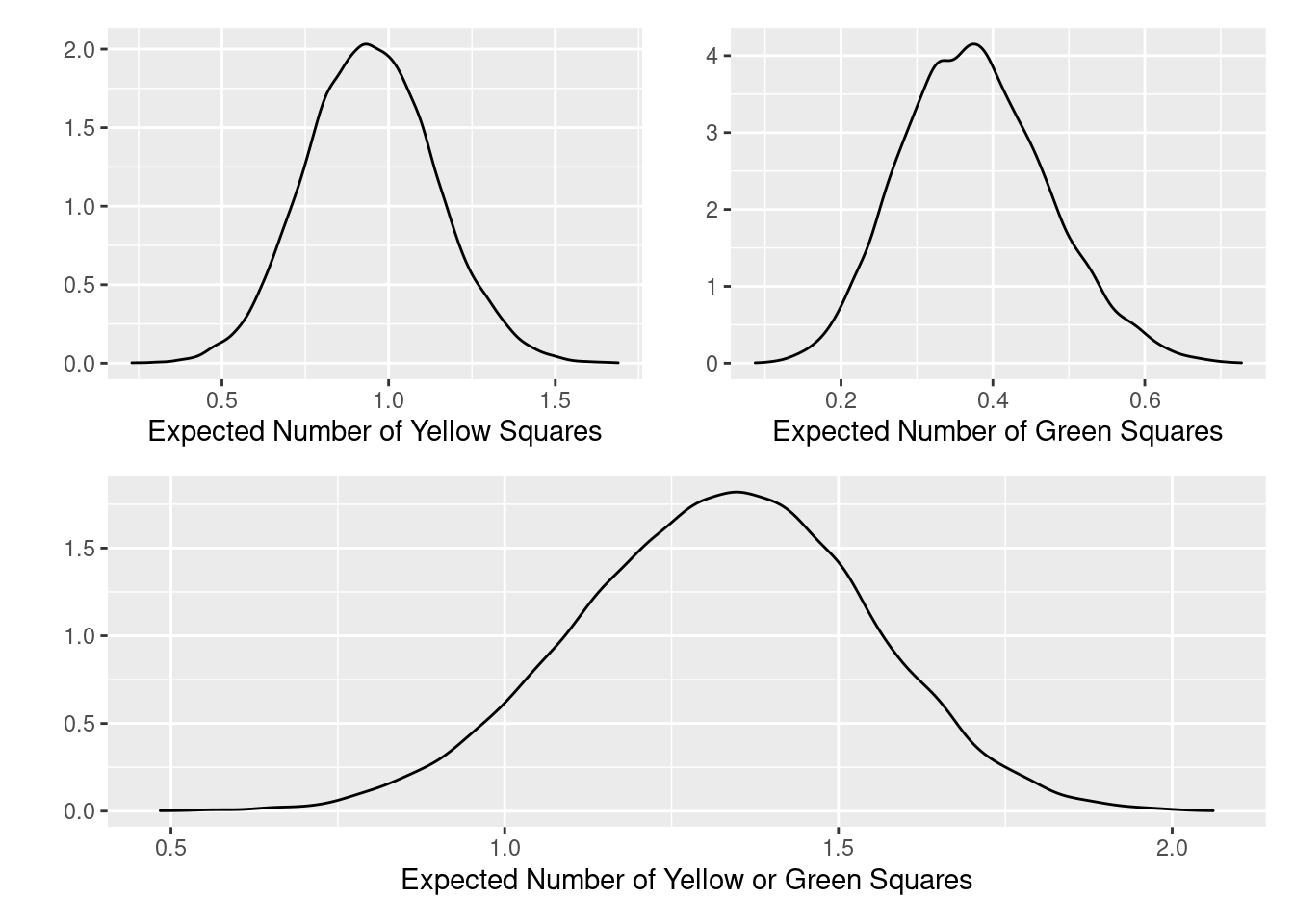
We can look at the distribution of expected values:

density_yellow <- word_values %>%
  bind_rows() %>%
  ggplot(aes(x = expected_yellow)) + 
  geom_density() + 
  labs(x = "Expected Number of Yellow Squares", 
       y = "")

density_green <- word_values %>%
  bind_rows() %>%
  ggplot(aes(x = expected_green)) + 
  geom_density() + 
  labs(x = "Expected Number of Green Squares", 
       y = "")

density_either <- word_values %>%
  bind_rows() %>%
  ggplot(aes(x = expected_green + expected_yellow)) + 
  geom_density() + 
  labs(x = "Expected Number of Yellow or Green Squares",
       y = "")

(density_yellow | density_green) / (density_either)

Clearly some words perform better than others as the first guess word.

The best words for yielding yellow squares are:

word_values %>%
  bind_rows() %>%
  mutate(word = five_letter_words) %>%
  top_n(5, expected_yellow) %>%
  arrange(desc(expected_yellow)) %>%
  select(word, expected_yellow)

## # A tibble: 5 × 2
##   word  expected_yellow
##   <chr>           <dbl>
## 1 assai            1.69
## 2 esere            1.67
## 3 asana            1.65
## 4 essee            1.65
## 5 anasa            1.64

These make sense: both “a” and “e” are common vowels (and the two most common letters in the English language) and “s” is a common ending letter for plurals.

The worst words for yielding yellow squares:

word_values %>%
  bind_rows() %>%
  mutate(word = five_letter_words) %>%
  top_n(5, desc(expected_yellow)) %>%
  arrange(expected_yellow) %>%
  select(word, expected_yellow)

## # A tibble: 5 × 2
##   word  expected_yellow
##   <chr>           <dbl>
## 1 fuzzy           0.230
## 2 wuzzy           0.246
## 3 buzzy           0.253
## 4 muzzy           0.298
## 5 fuffy           0.306

Again, those make sense - “y,” “u,” and “z” are all going to be uncommon letters.

Looking at gaining green squares:

word_values %>%
  bind_rows() %>%
  mutate(word = five_letter_words) %>%
  top_n(5, expected_green) %>%
  arrange(desc(expected_green)) %>%
  select(word, expected_green)

## # A tibble: 5 × 2
##   word  expected_green
##   <chr>          <dbl>
## 1 sanes          0.727
## 2 sales          0.716
## 3 sores          0.710
## 4 cares          0.708
## 5 bares          0.704

These words make sense, ending with “es,” a common ending in plurals.

The worst five:

word_values %>%
  bind_rows() %>%
  mutate(word = five_letter_words) %>%
  top_n(5, desc(expected_green)) %>%
  arrange(expected_green) %>%
  select(word, expected_green)

## # A tibble: 5 × 2
##   word  expected_green
##   <chr>          <dbl>
## 1 oghuz         0.0869
## 2 enzym         0.0992
## 3 zmudz         0.109 
## 4 iddhi         0.110 
## 5 ewhow         0.113

I am unsure that those are even words but I feel like all would be worth a lot in Scrabble (note: I have no idea how Scrabble is played but “ewhow” is a really weird word).

Now, the moment of truth, what are the best words:

word_values %>%
  bind_rows() %>%
  mutate(word = five_letter_words,
         combined_performance = expected_yellow + expected_green) %>%
  top_n(5, combined_performance) %>%
  arrange(desc(combined_performance)) %>%
  select(word, combined_performance, expected_yellow, expected_green)

## # A tibble: 5 × 4
##   word  combined_performance expected_yellow expected_green
##   <chr>                <dbl>           <dbl>          <dbl>
## 1 areae                 2.06            1.63          0.428
## 2 eases                 2.04            1.43          0.605
## 3 arase                 2.01            1.61          0.402
## 4 areas                 2.01            1.50          0.508
## 5 essee                 2.01            1.65          0.355

“areae” is your best bet although “areas” and “eases” seem like good contenders as well. I also confirmed that “areae” will be accepted by Wordle’s word list.

Online, people have suggested “weird,” “adieu,” and “heals” as candidate optimal first words. How do these compare against “areae?”

word_values %>%
  bind_rows() %>%
  mutate(word = five_letter_words,
         combined_performance = expected_yellow + expected_green) %>%
  arrange(desc(combined_performance)) %>%
  mutate(
    rank = row_number(), 
    pct = (1 - rank / n()) * 100
  ) %>%
  filter(word %in% c("areae", "weird", "heals", "adieu")) %>%
  select(word, rank, percentile = pct, combined_performance)

## # A tibble: 4 × 4
##   word   rank percentile combined_performance
##   <chr> <int>      <dbl>                <dbl>
## 1 areae     1      100.                  2.06
## 2 heals  1160       92.7                 1.63
## 3 adieu  2354       85.2                 1.55
## 4 weird  9728       38.9                 1.27

Based on this approach, “areae” is clearly better but “heals” and “adieu” seem worth considering. “weird” performs much more poorly at the 39th percentile of words, likely because the opportunity cost of the “w.”

Of course, all of this assumes that getting “not in the word” results has no value. Learning that a word doesn’t contain “e” might be as useful as learning that it is does. But that’s a level of complexity that I am not willing to deal with. Someone who really loves Wheel of Fortune and word games can take care of that.