Selection bias and observed values
I’m a man of a certain age and friend set, which means that I play a tabletop pen-and-paper roleplaying game called Pathfinder (similar to Dungeons and Dragons). You have a character with different values for strength, dexterity, constitution, charisma, wisdom, and intelligence. The values for these scores are generated by rolling dice. Specifically, for each score, you roll four d6 (six sided dice), remove the lowest die, and sum the three remaining dice. You roll a set of six stats twice and then pick which collection gives you the better set of numbers.
For instance, if I rolled four dice and got a 3, 5, 2, 6, I’d remove the 2 and add the 3, 5, and 6 to get my score of 14. I’d repeat this process 5 more times to get my set of six scores for my first set of rolls. I’d then repeat the process to get another collection of stats.
We also allow a person with a set of bad stats to let the person running the game to re-roll for them. If you take this option, you must take the new rolls, even if they are worse than the better of your two sets.
This creates an interesting result where the player stats are better than expected. To see this, at least in a simulation, let’s define a function to roll a single stat (4d6, remove the lowest die, and sum):
library(tidyverse)
library(gtsummary)
roll_stat <- function() {
  values <- sample(1:6, 4, replace = TRUE)
  score <- sum(values) - min(values)
  return(score)
}
And another function that runs the set of six statistics:
roll_set <- function() {
  rolls <- replicate(6, roll_stat())
  sum_of_rolls <- sum(rolls)
  return(sum_of_rolls)
}
We then want to make a function to roll a character’s statistics by generating
two sets and taking the better of the two. Additionally, we want to allow for
players to opt into having the GM re-roll for them. We’ll have the probability
of opting into a GM re-roll equal to the probability that a random roll is
better than the current best set for the player. This is operationalized as
1-pnorm(best_roll, 72.5, 6.9) where the 72.5 mean and 6.9 standard deviation
come from a Monte Carlo simulation of 1,000,000 random rolls. The GM re-roll
option can be totally turned off as well.
roll_character <- function(gm_reroll) {
  set_1 <- roll_set()
  set_2 <- roll_set()
  stats <- max(c(set_1, set_2))

  if (gm_reroll) {
    if (rbinom(1, 1, pnorm(stats, 72.5, 6.9, lower.tail = FALSE))) {
      stats <- roll_set()
      roll <- "gm"
    } else {
      roll <- "player"
    }
  } else {
    roll <- "player"
  }

  results <- tibble(stats = stats, roll = roll)
  return(results)
}
We then generate a bunch of rolls, a bunch of characters with and without the ability to have the GM reroll your stats:
set.seed(96312)
k <- 100000
distribution_of_rolls <- replicate(k, roll_set())
distribution_of_characters <- bind_rows(replicate(k, roll_character(gm_reroll = FALSE), simplify = FALSE))
distribution_of_characters_with_reroll <-  bind_rows(replicate(k, roll_character(gm_reroll = TRUE), simplify = FALSE))

outcomes <- tibble(
  stats = c(distribution_of_rolls, distribution_of_characters$stats,
            distribution_of_characters_with_reroll$stats),
  label = rep(c("Fair Roll", "Without GM Reroll", "With GM Reroll"), each = k),
  roller = c(rep("Fair", k), distribution_of_characters$roll,
            distribution_of_characters_with_reroll$roll)
)
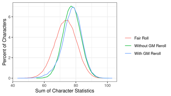
Next, we visually inspect the distribution of the character stats:
outcomes %>%
  mutate(label = forcats::fct_relevel(label, "Fair Roll", "Without GM Reroll")) %>%
  group_by(label, stats) %>%
  count() %>%
  group_by(label) %>%
  mutate(pct = 100 * n / sum(n)) %>%
  ggplot(aes(x = stats, y = pct, color = label)) +
  geom_line() +
  labs(x = "Sum of Character Statistics",
       y = "Percent of Characters",
       color = "") +
  theme_bw()
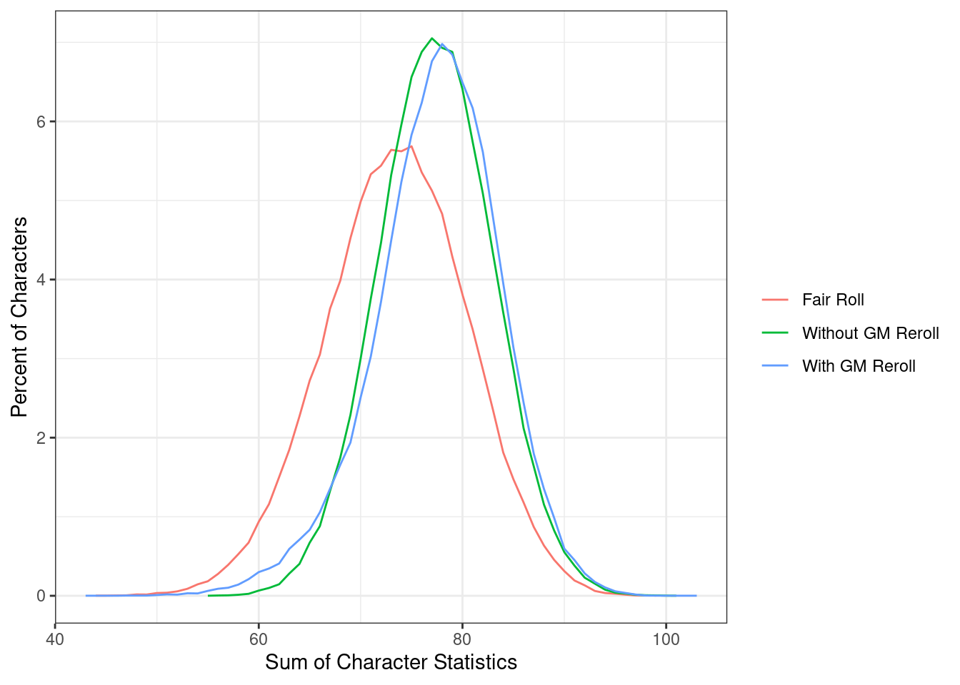
We can see the “Without GM Reroll” and “With GM Reroll” distributions are shifted towards much higher stats than the “Fair Roll” distribution - depite the fact that they are all the results of a fair roll.
tbl_regression(lm(stats ~ label, data = outcomes))
| Characteristic | Beta | 95% CI1 | p-value |
|---|---|---|---|
| label | |||
| Fair Roll | — | — | |
| With GM Reroll | 4.0 | 3.9, 4.0 | <0.001 |
| Without GM Reroll | 3.9 | 3.8, 4.0 | <0.001 |
| 1 CI = Confidence Interval | |||
Compared to the “Fair Roll,” player stats are 3.9 points greater. Adding the GM re-roll option increases the average score by another 0.09 points. Why does this happen?
Relative to the “Fair Roll,” we are only seeing the “winners.” The person rolls the dice to generate two sets of values under the same “rules” both times; however, they select the better of the two values. This causes the observed value to exceed and have a different distribution than a Fair Roll. Adding the option for a GM reroll increases it again because players unhappy with their of their rolls, likely because they are too low, will opt into having the GM reroll their stats. Since only players likely to benefit from this choice make this choice, this again increases the average player stats.
This causes problems for inference. For instance, having the GM reroll the stats simply replaces your numbers with the results drawn from a fair roll condition. However, we know that a fair roll is worse than the condition without the GM reroll, so how does the GM replacing your stats with a fair roll improve the outcome? It does so because it selectively replaces values improbably low with new draws but does not replace high values. This shifts the lower end of the distribution but not the upper end, moving the mean to a larger value.
Additionally, if we wanted to know if the GM was a “luckier roller” than the players, we might consider regressing the player stats on an indicator for whether they were rolled by the player or the GM:
lm(stats ~ roller,
   data = outcomes %>%
     filter(label == "With GM Reroll")) %>%
  tbl_regression()
| Characteristic | Beta | 95% CI1 | p-value |
|---|---|---|---|
| roller | |||
| gm | — | — | |
| player | 5.6 | 5.6, 5.7 | <0.001 |
| 1 CI = Confidence Interval | |||
The player rolled stats are an average of 5.6 points higher than the GM rolled stats. Is the GM just bad at rolling? No, again, the choice to reroll depends directly on the quality of the roll. The people who opted out of a reroll are not valid counterfactuals of those who elected to have a reroll.
In the real world, we often only observe outcomes that are realized. If we were studying wages, for instance, we might observe the wage conditional on a person accepting a job offer. We would see a wage that is inflated compared to the underlying offers because the person is selecting only jobs that have greater wages. We would find that people holding out for an uncertain third job offer, declining the first two, would make less - but that behavior could easily be the result of the first two offers being poor.
We are typically interested in the “underlying” dependent variable but often what we observe in real-world data is some manifestation of that variable with some, or potentially many, selection effects happening first. Understanding the relationship between your confounders, your indepdendent variable, and the dependent variable is critical.